Learning Environment Simulators from Sparse Signals (my Masters thesis)

I spent most of 2017 on model-learning for planning from sparse signals. The complete thesis is available here, and the corresponding code is available here.

This post is intended as a friendly introduction to the idea I explored in my thesis. In part 1, I offer motivation for why one might want to learn an environment model from sparse signals like an agent’s reward. In part 2, I’ll give an overview of the method itself, and some of inherent virtues and drawbacks. In part 3, I’ll discuss the benchmark environments I created to evaluate the method, and a few of the actual results.

Motivation

I spent my Masters thesis trying to answer the following question:

Imagine I want to teach a robot to play baseball on the field by my house. My robot has a camera, a bat-swinging mechanism, and a computer to manage the two. That’s it.

Now, initially, my robot does not understand baseball, or anything else.

It doesn’t know how to measure how fast a baseball is moving towards it (velocity estimation).

It doesn’t know that baseballs accelerate downwards over time (gravity).

It doesn’t know that baseballs exist continuously (object permanence).

It doesn’t even know what a baseball looks like, or why it matters.

It only knows three things:

1. What the world around it looks like (a sequence of images)
2. What it did with the bat (a sequence of actions)
3. Whether its coach says it did a good job, or a bad job (a sequence of rewards)

The robot really wants to learn how to play baseball. And we want our little robot child to succeed. So what do we do?

Well, one solution would be model-free reinforcement learning. In effect, this means letting the robot swing and swing and swing. Whenever the coach says it did good, it’ll try to figure out what was special about that situation, and then repeat that action in similar situations in the future. (Vice-versa if the coach yells at it.) Unfortunately, learning baseball by swinging wildly and blindly until you succeed can take a very, very long time.

A different, perhaps more efficient approach would be to let the robot watch lots of hours of baseball, perhaps played by other robots, and to let it try to learn the rules of baseball (and of physics). We’re going to define “knowing the rules” loosely as the ability to simulate, given the current state of the robot (e.g. camera image) and a choice of action (bat swing), what the next state is likely to look like, and whether the coach will praise that action. Once our robot knows the rules of baseball, it can play out the short-term future in its head and choose the action that, by its rules, will lead to its highest reward.

This is known as model-learning or predictive learning, and is the type of method we’ll focus on here.

Now, the most common method of visual model-learning is pixel-level image reconstruction. That is, the robot aims to learn to predict each pixel in the new image from the pixels in the previous image (as well as the previous action). The accuracy/inaccuracy of every pixel is weighted equally, and the goal is to minimize this inaccuracy and to reproduce the whole future image.

This sounds good in theory, but let’s for a moment step back onto our baseball field.

Imagine the trees behind the robot are blowing wildly in the wind, and there are people running around in the background. Or worse, imagine our robot is suddenly forced into the major leagues, and sees thousands of people in different colored shirts bustling around doing all sorts of things. Our robot’s goal is to accurately reconstruct the entire image, so it’s going to spend a ton of effort trying to learn how to model the motion of the trees and of the people.

In all of the hustle and bustle, it might end up ignoring the relatively small white blob of the baseball. Without identifying the baseball, it’ll have no chance to learn the rules of the game.

So somehow, we’ve got to make sure the robot learns to focus on the baseball. One option is to explicitly hint to it that the baseball’s position is important, or to provide the robot some other new information to focus its model-learning. In practice, such approaches might end up being easier and more time-efficient.

But in theory, our robot actually already has enough information to realize the baseball is important. That’s because, if the robot were paying attention, the only times its coach says that it did good or bad was when that white blob of pixels was right nearby us. If we focused on predicting the reward (the coach’s response), both for the next image frame and for several future frames, we’d quickly realize that modelling the movement of the baseball is essential. Almost everything else, from the swaying trees to the bustling crowd, might be important in pixel prediction, but in reward prediction, we’re only incentivized to model the vital elements of the world.

This is the core idea explored in my Master’s thesis. What if we tried to learn a representation of the environment, and a transition model for the environment, whose primary objectives are accurately predicting multi-step reward?

Learning Environment Simulators from Sparse Signals

Let’s recap, more rigorously:

Given a series of historical environment sequences {o_t, a_t, r_t, o_t+1}_n (observations, actions, rewards, and future observations respectively), we would like to find a state representation s_t = E(o_t) and transition model s_t+1, r_t ~ T(s_t, a_t) that best predict, given an initial state s_t and a sequence of actions a_t, a_t+1, a_t+2, …, the sequence of resulting future rewards r_t, r_t+1, r_t+2, …

(Side note: we use “rewards” (r) and “goals” (g) interchangeably - a “goal” is just a type of reward that occurs once at the end of an episode.)

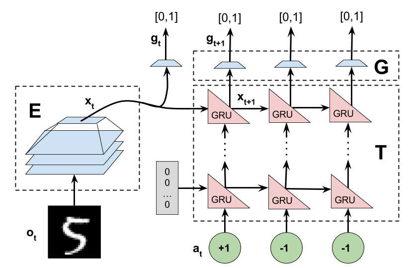
In practice, we model the encoder E and transition function T as neural networks (splitting the reward-prediction component of the transition model into a separate network G). the rewards are predicted for a fixed k timesteps into the future.

One important benefit of this approach is that we are never required to construct a decoder, i.e. an inverse encoder that maps from the latent state s to a corresponding observation o. This is particularly useful for those domains in which no such decoder exists, like rendering the crowd in the background of a baseball game. Some work has used generative modeling to avoid the need to have a perfect-fidelity decoder, but GANs are hard to train, and this still requires the latent state s to contain sufficient info to reconstruct the next state. In our model, the learned s = E(o) can be sparse and model only the portions of the state necessary to predict the reward.

State Consistency Loss

There are a few modifications necessary to make the learning process work, one of which is adding a “state consistency loss”. That is, if I extract a latent state s_t from an observation o_t and then simulate it forward k timesteps to get an approximation of s_t+k, the result should be roughly the same as if I had extracted the latent state from E(o_t+k) directly.

This is necessary for the following reason. Imagine a simple environment in which the “observation” is a number between 1 and 100, and there’s only one action, called “increment”, which increases the number by 1. The game ends, and the agent gets reward 1, when the number reaches 100. (Otherwise the reward is 0.) Now, the agent only learns to predicts reward for a 3-action horizon. So, the agent may construct a fully-valid representation s = E(o) that uniquely identifies states 97 (reward in 3 steps), 98 (reward in two steps), 99 (reward in one step), and sets every other observation (from o=1 to o=96) to be the same latent state. Because as far as the agent is concerned, both for o=96 and o=1, it never observes a reward within 3 timesteps.

To fix this glitch, we simply enforce that in addition to accurately predicting reward r_t+i, the agent accurately predicts the future low-dimensional state s_t+i+1. This means that s₉₆ = E(o=96) will be observably different from s₁ = E(o=1), because in the next step, s₉₆ will yield s₉₇ (which we had already uniquely identified). By repeatedly enforcing this consistency condition, we bootstrap to eventually uniquely represent every one of the hundred original states.

An interesting implicit assumption is that states contain only information relevant to reward-prediction. That is, given two initial states, if executing any sequence of actions yields the same reward for both states, then those states are functionally identical. While this may seem like an undesirable result, it theoretically ensures that the state representation is sufficient to choose the optimal next action to maximize reward. (However, were the reward function to change, the state representation might become useless.)

One drawback of this solution is that the longer the sequence of states defined only with respect to other states (and not to some sort of reward), the weaker the signal being provided to the earliest states. Both the usefulness the state consistency loss, and its drawbacks, are experimentally validated in Chapter 3 of the thesis.

Sidebar: This Can’t Possibly Work

The first thing to note about this proposed learning problem is that it is really, really hard. Despite the introduction’s optimism, it is near-impossible for an agent to learn a model for a complicated environment only by being told post-game whether it performed well or not. Imagine learning the physics of pole-vaulting by looking at the track, closing your eyes, running forward while swinging your pole randomly, and then being told how high you went.

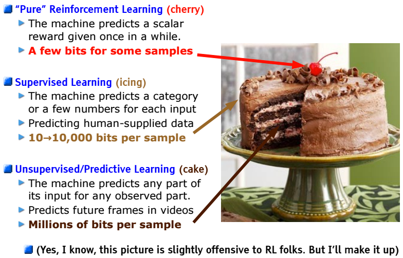
In a sense, this approach suffers from the same criticism that Yann LeCun famously lodged against model-free RL. The reward simpy doesn’t offer enough signal to efficiently learn an environment model, meaning the approach is destined to fail in real-world systems.

However, I think there is something to learn from thinking about model-learning from sparse signals, if only as a thought exercise.

Environment-learning today is focused on using massive input signals (prior images) to predict massive future signals (future images), and the act of “learning” is the process of squeezing in as much of the high-dimensional inputs as you can into lower-dimensional representations that can be simulated forward with minimal information loss, and then decoded back into a high dimensional image. In a sense, the “learning” is about maximizing the amount of information encoded into the state.

Our approach tackles a fundamentally different type of learning problem. Here, we use large input signals to predict sparse future signals - so sparse, in fact, that an agent might not receive any signal (reward) at all for several timesteps after the observation. As a result, the learned state representation is initially sparse as well, as the learner has little signal compelling it to construct a complex state representation. The act of “learning” becomes a process of backsolving each signal, beginning from the simplest state representations (those right before a possible signal/reward event) and slowly growing in complexity (finding states that lead to states that lead to reward events, and so on). In this sense, learning a simulator from sparse signals is less about distilling the signal from the noise and more about recursively constructing more complicated state representations. Whether or not such a capability is tractable for modern deep learning, it is a different learning paradigm that I found interesting to explore.

We can also make the approach more tractable by providing denser (yet still sparse) signals than environment reward, as discussed in Chapter 4 of the thesis. These auxiliary signals are often already vailable, like GPS or classical odometry on a robot. By studying the simplest, harshest case of sparse-signal model-learning (pure-reward), we can hopefully extract insights that will generalize to these more complicated and realistically-applicable cases.

Benchmark environments and a few results

To demonstrate the abilities and trends in such an approach, we need some simple benchmark environments. These environments should:

• have an interpretable true latent representation (if we can find it)
• have deterministic transitions in “true state” space (to avoid dealing with branching states; for more, see Chapter 1 of the thesis)
• have a simple “encoder” mapping (from o to s), but no simple decoder mapping (from s to o)
• have sparse rewards

I created several such environments, implemented using the OpenAI gym interface. The code is available here.

One such environment is what we’ll call the “MNIST game”.

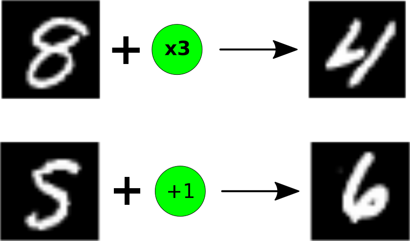
The logic of the game is simple: each observation is a digit (e.g. an image of a 5) from the MNIST dataset, corresponding to the environment’s true hidden state (e.g. 5). Each action is a simple arithmetic operation mod 10. For example, the “+1” action would take an MNIST image of a 5, and convert it to an image of a 6, as in the above figure. The environment starts at a random digit, and the goal is always to get to 0 (upon which the agent receives a reward of 1, and the episode ends).

One nice attribute of this game is that we can easily change the gameplay dynamics by changing the legal transitions. So for example, allowing only “+1” and “-1” would yield a simple strategy (increment when above 5, decrement otherwise). On the other hand, a more complicated set of actions (“+1”, “+0”, “x2”, “x3”) yields a substantially more involved strategy.

Importantly, the “observed” MNIST digit image is drawn randomly from the set of all MNIST images of that digit. So while finding an “encoder” mapping from the observation to the true state is as easy as solving MNIST, finding a decoder to map from the latent state to the observation is hard. (A GAN could do it, but GANs are “hard”.)

When we train our environment model on the simple (“+1, -1”) MNIST game, and then visualize the learned state embeddings use their top 3 principle components, we get something like this:

This shows the state representation of a model trained to predict reward 3 timesteps ahead. Top left: states directly encoded from observations; Top right: states simulated forward 1 timestep; Bottom left: states simulated forward 2 timesteps; Bottom right: states simulated forward 3 timesteps.

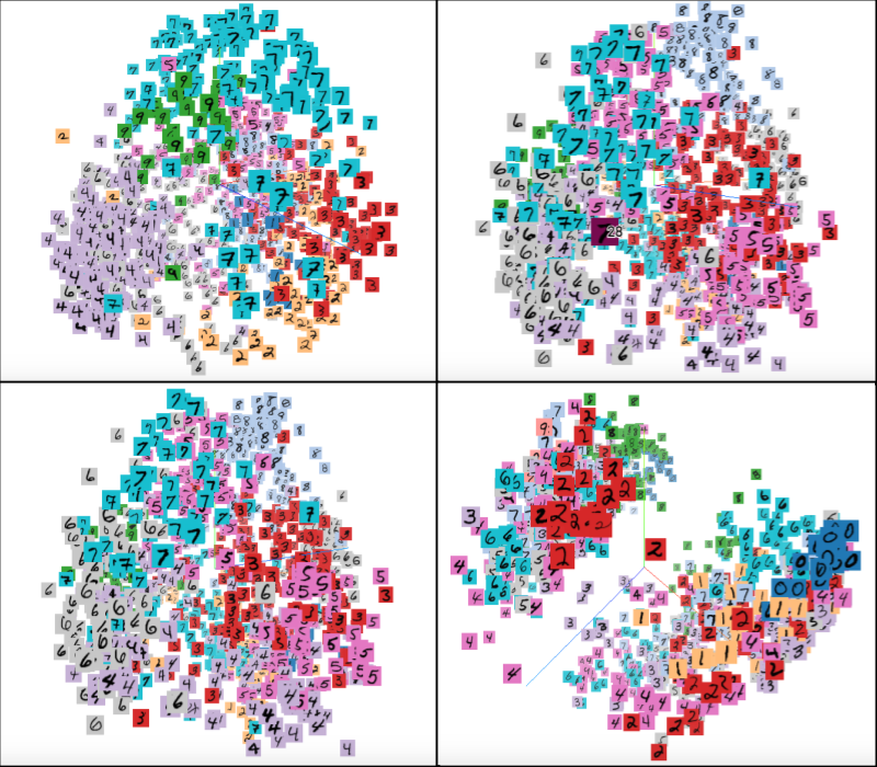
As we can see, the model actually learns a high-quality encoder which initially separates the different latent states out quite nicely (learning only from their similarity in future rewards given similar actions). However, after each timestep, the quality of the embedding degrades (implying the transition function is unreliable) until at the end of the prediction horizon (the third step) the embeddings appear jumbled together. That said, a pocket of 0s and 1s, corresponding to the rewarded state and thus easily distinguishable, is still visible.

This suggests that while the learner is able to distinctly identify each of the states originally, the farther forward in time it simulates the state, the worse the state will be. However, it’s difficult to get a quantitative understanding of the learned state representations by eyeballing their principle components.

To get a better sense of how well the model is learning the data clusters, I used the following measure. First, I took a group of state representations (e.g. states simulated 3 steps from first encoding) and ran kmeans to get a rough approximation of the 10 clusters that represent the data. Then, I computed the normalized mutual information between the learned clusters and the true latent states (which I kept track of without informing the learning algorithm). The result is a metric approximately proportional to how well the learned model distinguishes between future states that are truly different.

Below are the plots of this “NMI score” over simulated time, for environment models trained to predict reward/state consistency a variable number of timesteps k into the future. (This time, the MNIST game is more complicated, with +1, 0, x2, and x3 all possible actions.)

The NMI scores for varying prediction-length environment learners.

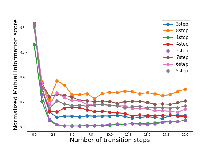
We can clearly see that all the learners accurately determine the initial state encodings (which is unsurprising, as MNIST is fairly easy to learn). However, over time, the learners with the longer prediction horizon consistently outperform those with shorter horizons (and this trend holds even beyond their fixed-length prediction windows). This might be because predicting longer trajectories requires finding repeated patterns of states. The results of this experiment suggest that our models are in fact learning generalizable environment dynamics.

Finally, we can evaluate the functional quality of our learned environment models by integrating them into a real planner and trying to plan. We use a simple BFS planner that uses the environment simulator to look up to 5 timesteps into the future. It ultimately chooses the path with the highest assigned probability of reaching the goal. Below, we plot its success rate in reaching the goal within the first 5 steps (again varying trained prediction length k).

The success rates for BFS planners using learned environment models with variable training horizon. ‘Simple’ refers to the simple MNIST game (+1, -1) and ‘complex; refers to the complex MNIST game (+1, +0, x2, x3).

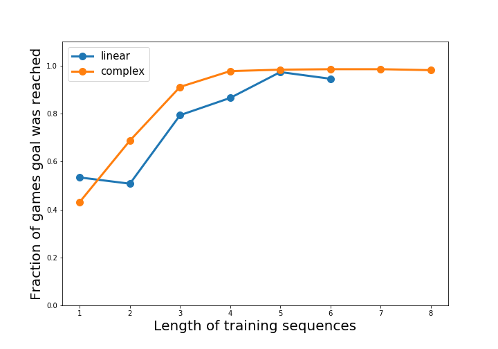
We can see that, beyond the shortest-horizon learners, nearly all of the learned models are able to consistently lead the agents to the goal.

So, the MNIST game is solvable by an agent aiming to exclusively do reward prediction. While this is an extremely simple example, it clues us into some of the trends of learning simulators from sparse signals. Longer training-horizons are vital for planners to generalize well. The structure of the environment’s transitions affect its learnability. And the closer a state is to a signal/goal, the more likely it is to be accurately predicted by the environment model.

For many more experiments and results, and a deeper mathematical treatment of the algorithm, you can check out the thesis. (Have I plugged it enough?)

So, this might not be the satisfying answer our robot was looking for. He may need to wait another day before he can learn the rules of baseball from observation and coach-screaming alone. But hopefully he has at least learned that there is useful information in his coach’s advice, if only he’d stop yelling.

Yours, Yo